
From Telephones to Transformers: A Brief History of Quantization
Model quality used to be AI’s limiting factor. Now, it’s model economics. Where cost per token, watts per rack, and tokens per second dominate the conversation, no topic is more pertinent than model optimizations. And, in that conversation, few optimizations are as well-known, and as misunderstood, as quantization.
In ML, quantization is a technique to reduce computational and memory costs by converting a model’s weights and activations from higher-precision data types (e.g., FP32) to lower ones (e.g., INT4). Today, many techniques and formats exist. For developers, the challenge is knowing which one best fits their implementation.
What follows is a brief history of quantization, from its origins in 19th-century numerical analysis to the latest research today. With this history, developers and hardware architects alike can better judge the available methods and anticipate where the next round of efficiency gains will come from.
Origins in signal processing
Quantization predates machine learning by about a century. Mathematicians first arrived at it when trying to represent continuous quantities in systems that could only store discrete values.
Many trace the first formal treatment to W.F. Sheppard, a statistician working with binned data. He noticed that binning itself corrupted his results, and that computing a variance from grouped data gave a systematically wrong answer because every value had been nudged to the center of its bin. His 1897 analysis worked out how large that error was and how to correct for it. In the history of quantization, this work introduced the idea that rounding error was not random noise, but had a predictable size.
Claude Shannon put the question on formal footing fifty years later. His problem at Bell Labs was scarcity, since a telephone line could only carry so much, and engineers needed to know how much information they could push through it. His 1948 coding theory work showed that the answer depends on the message's statistics. A system wastes capacity when it spends as many bits on a common event as on a rare one, so an efficient design allocates bits by probability. Quantization inherited the principle.
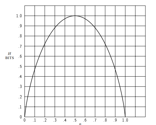
Figure 1: Entropy in the case of two possibilities with probabilities p and (1 p). (Source: Shannon et al).
He returned to it in 1959 when trying to determine how little distortion is achievable at a given bit rate. His distortion-rate functions work gave a theoretical floor and introduced vector quantization, which handles a group of values as one symbol instead of rounding each one alone.
However, the first practical algorithm came out of the telephone network. Moving the telephone network to digital transmission required pulse code modulation to digitize speech. Speech amplitude is not spread evenly across its range: quiet passages dominate and loud peaks are rare, so evenly spaced levels wasted most of their resolution on amplitudes the signal almost never reached. In response, Lloyd circulated a least-squares method in 1957 which assigned each sample to its nearest level, moved each level to the center of the assigned samples, and repeated until it was stationary. His paper was unpublished until 1982, by which point researchers had rediscovered the same procedure and named it “k-means”.
Work from this period formed the basis of the field.
Compressing features before compressing models
Neural networks were not the first systems to hit a memory wall. By the late 2000s, large-scale image retrieval faced a practical version of the same constraint, holding hundreds of millions of high-dimensional descriptor vectors that cost too much time and memory to compare in full precision.
The first widely accepted solution came from a paper that was not about compression at all. Indyk and Motwani introduced locality-sensitive hashing in 1998 to get around the “curse of dimensionality” in nearest-neighbor search. The concept is to project a vector through random hyperplanes and keep only the sign of each projection. This idea leverages the fact that vectors that sit close together in the original space tend to collide in the resulting binary signature.
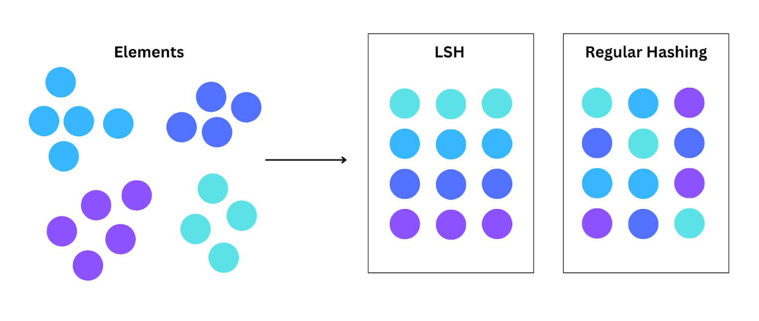
Figure 2: Locality-sensitive hashing versus regular hashing. (Source: Zilliz)
The result's durability came from constructing a representation whose geometry preserves a task-relevant notion of similarity. Because locality-sensitive hashing uses random projections chosen without ever looking at the vectors they encode, the natural next question was whether researchers could fit the representation to the data instead.
Jégou, Douze, and Schmid answered the question in 2011 with product quantization. This technique split the vector space into subspaces and gave each its own small codebook, so a handful of bytes indexes an enormous set of code points. Norouzi and Fleet went further in 2013 with Cartesian k-means, learning the decomposition itself.
Each step reinforced the finding that smarter mapping recovers more accuracy than arbitrarily increasing bit count.
The coordinate system becomes part of the quantizer
Next, Gong and Lazebnik made a meaningful observation in 2011 with Iterative Quantization. Instead of treating the original coordinate axes as fixed, they solved for a rotation that aligns the data with the quantization grid before applying the sign function. By rotating first, they cut binary encoding error on the same bit budget. A better coordinate system, it turned out, can also be more valuable than adding extra bits.
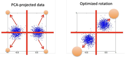
Figure 3: Binary codes assign each point a sign along every axis (left). Rotating the data first (right) moves most of it away from those boundaries and reduces encoding error.
In turn, their findings raised a cost question. A learned dense projection over a d-dimensional vector takes time and memory proportional to d squared, which erases the savings the compact code promised.
Researchers answered this challenge with structured transforms that constrain the rotation to a cheaper form. Gong and colleagues factored the projection into two smaller matrices with bilinear projections in 2013. Yu and colleagues constrained it to a circulant structure a year later, turning the multiplication into a convolution that the FFT executes in d log d time.
From features to model parameters
Today's chatbots make it easy to forget that for most of AI's history, the most intelligent system available was a search engine. People typed a question into Google and expected an answer good enough to act on, and the companies serving those queries got there by leaning on enormous amounts of data.
Back then, the models doing the work were comparatively small. Intelligence did not live in the parameters, but in the corpus. A model's job was to reach into that corpus and pull back something relevant. In that case, data was the engineering problem. Everything hinged on compressing a massive collection into a compact, well-structured form a system could search in milliseconds, which is why the field spent a decade refining the feature-compression methods above.
Some researchers took the idea to its logical end. Alyosha Efros at Berkeley argued that intelligence itself might fall out of this arrangement: store enough of the world's data, build a good enough mechanism for retrieving it, and k-nearest-neighbor search over that collection gets you most of the way to solving AI. In that view, intelligence is a retrieval problem.
Deep learning inverted the arrangement. Instead of keeping the data beside the model and searching it at query time, training absorbed the data into the model. The parameters became the corpus. A trained network consults no database of examples, only the weights those examples produced.
When the data lived outside the model, compression meant shrinking the dataset. Now that the data lives inside the weights, a query at inference is a search through the model itself, and the expensive part is reaching every parameter the answer depends on. The object worth compressing moved from retrieval features to the network's weights and activations, and the cost of access moved with it.
A focus on compression
With this new direction, Han and colleagues showed how far compression could go in 2016 with Deep Compression. This work packed pruning, trained quantization, and Huffman coding into one pipeline.
A more aggressive line of work explored whether a network could run on a single bit, with Hubara and colleagues training networks with 1-bit weights and 2-bit activations. Their efforts reached 51% top-1 accuracy on a quantized AlexNet, showing that bitwise operations could replace most runtime arithmetic.
Mohammad Rastegari and colleagues took the idea to ImageNet scale in 2016 with XNOR-Net, binarizing weights and convolutions and recovering much of the lost accuracy with one scaling factor per weight matrix. This work showed that quantization could be effective because it could maintain quality.
Those results changed the very premise of quantization. Rather than being a simple storage technique, it became part of the computational graph, which meant training had to account for it.
Jacob and colleagues consolidated the practical version in 2018 with an integer-arithmetic-only inference scheme they co-designed with its training procedure. Around that point, the field split into two camps:
Post-training quantization, which converts a trained model with no retraining and no labeled data.
Quantization-aware training, which folds the rounding into the training loop and reaches lower bit-widths at the cost of fine-tuning.
Which error matters?
Every method above aims to minimize the distance between a weight matrix and its quantized copy. Researchers eventually realized that, since layers contribute outputs to the network, what really matters is the error in the layer’s output, not the error in weights themselves.
Frantar and colleagues made that distinction practical in 2023 with GPTQ. This work uses second-order information from the layer Hessian to quantize weights column by column, then updates the remaining columns to compensate. The method brought accurate post-training quantization to transformers at a scale where retraining wasn’t feasible.
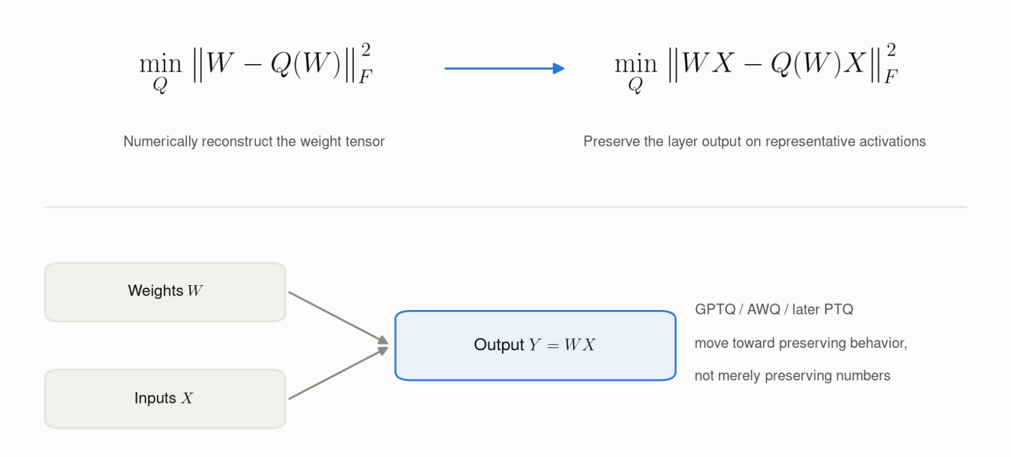
Figure 4: Weight-space reconstruction error and functional output error are not equivalent objectives.
Lin and colleagues sharpened the same insight from the activation side with AWQ in 2023. Not all weight channels matter equally, and activation statistics reveal which ones carry the salient signal. Keeping about 1% of channels in higher precision recovers most of the lost accuracy, but mixed-precision layouts run poorly on real hardware. As such, AWQ rescales those channels instead and quantizes everything uniformly.
Xiao and colleagues took the complementary route with SmoothQuant in 2022, dividing activations by a per-channel scale and multiplying weights by the same factor. The reparameterization shifts the difficulty to the tensor best able to handle it, making 8-bit weight and activation inference practical.
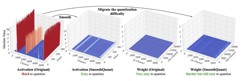
Figure 5: SmoothQuant divides activations by a per-channel scale and multiplies the weights by the same factor
Rotations return at a new scale
During these developments, rotation had been sitting in the literature for over a decade before language models made it urgent again.
Ashkboos and colleagues brought the coordinate-system idea back to large language models in 2024 with QuaRot. This research used computational invariances and Hadamard rotations to spread activation outliers evenly and unlock 4-bit inference. Liu and colleagues followed with SpinQuant, which learns the rotations instead of drawing them from a fixed family. Sun and colleagues extended the line with FlatQuant, using learned affine transforms held together by structured decomposition and fusion to keep the transform executable at inference time.
Bits and budget
Today, the phrase “4-bit quantization” is a catchall term, but it hides how much variation can exist within four bits. For example, INT4, FP4, NF4, and NVFP4 differ in their code points, scaling rules, block sizes, dynamic range, and hardware mapping. Four bits only truly names the storage budget, but designers must also consider scaling granularity, outlier handling, accumulation precision, and the kernel that executes the result.
Weights were the obvious first target for quantization because they are static and easy to reason about. But as models scale, activations and the key-value cache dominate inference memory and bandwidth as much as parameters do. Zirui Liu and colleagues showed with KIVI in 2024 that KV-cache quantization can reach 2 bits by treating keys and values asymmetrically. This work lowered memory pressure and increased the batch size a server can hold. Microsoft Research's BitNet work goes further upstream, designing architectures around 1-bit weights instead of converting a trained model to low precision afterward.
Today’s ceiling
The history of quantization is remarkably consistent.
LSH asked which projection preserves similarity.
Product quantization asked how to partition a space.
ITQ asked which rotation makes binary codes easier.
XNOR-Net asked whether the network itself could compute in a binary domain.
GPTQ asked which weight errors matter at the layer output.
AWQ and SmoothQuant asked how activation statistics should reshape precision.
QuaRot and SpinQuant returned to the coordinate system.
Microscaling and NVFP4 made the scaling hierarchy part of the format.
KV-cache quantization expanded the target to runtime state.
The next question is larger: what computation should exist for the representation the model actually wants.
Quantization started as a way to compress information. It is becoming a way to shape computation around intelligence. That is the long arc—and it points toward a future in which intelligence shapes compute.
