AI Inference at Scale Depends on Memory and Storage, Not Just Compute
Every company that deploys AI at scale eventually faces the same question. What hardware should it buy, and how should that hardware be arranged?
Most teams start with the model. They pick an LLM, estimate how many GPUs it needs, and plan the fleet around that number.
But what if we told you that the model is only part of the answer? What if two teams with the same hardware and model could achieve wildly different results? And what if, as it turns out, the difference comes down to memory and storage, not just compute?
This article explains why this is the case, and shines new light on planning for the next generation of AI infrastructure.
But first, we must start with the basics.
Two Jobs Behind Every AI Answer
To start, consider what happens when someone sends a prompt to a large language model (LLM). During inference, the model does two different jobs.
First, the model reads. It takes in the whole prompt, which could be one sentence or an entire codebase, and works out what every token means in context. Because the whole prompt already exists, the GPU can process all of its tokens at once. Engineers call this step “prefill.”
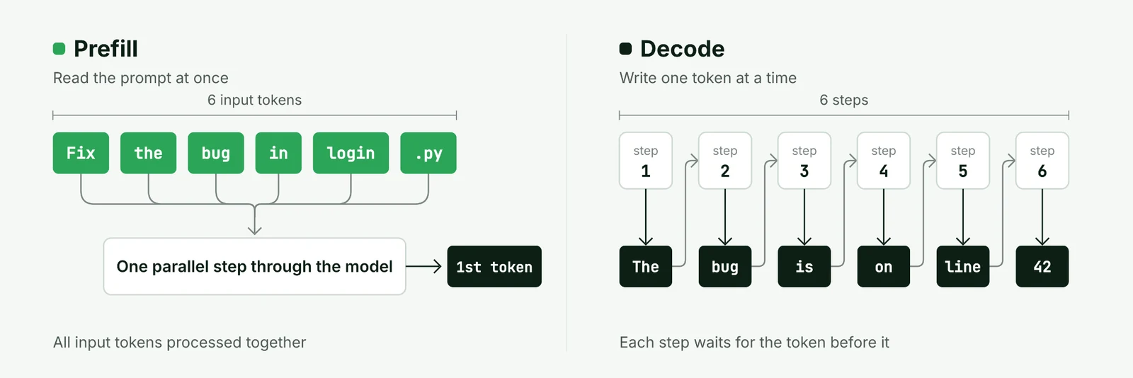
Figure 1: During prefill, the model processes every input token in one parallel step. During decode, the model writes output tokens one at a time, and each step waits for the previous token.
Then, the model writes. It produces the answer one token at a time, and each new token depends on the ones before it. So, the model can’t start the second token until the first one exists. Engineers call this writing step “decode”.
Two Jobs, Two Different Bottlenecks
Although prefill and decode run the same model, the two inference jobs stress the hardware in opposite ways.
To compute anything, a GPU moves the model's weights, the billions of numbers that make up the model, from memory into its arithmetic units.
During prefill, the whole prompt already exists, so one pass can process every input token at once. For a 142,000-token prompt, the GPU streams the weights once and uses each weight 142,000 times. Because parallel processing is possible, prefill speed depends on how many arithmetic units are available and how fast those units are.
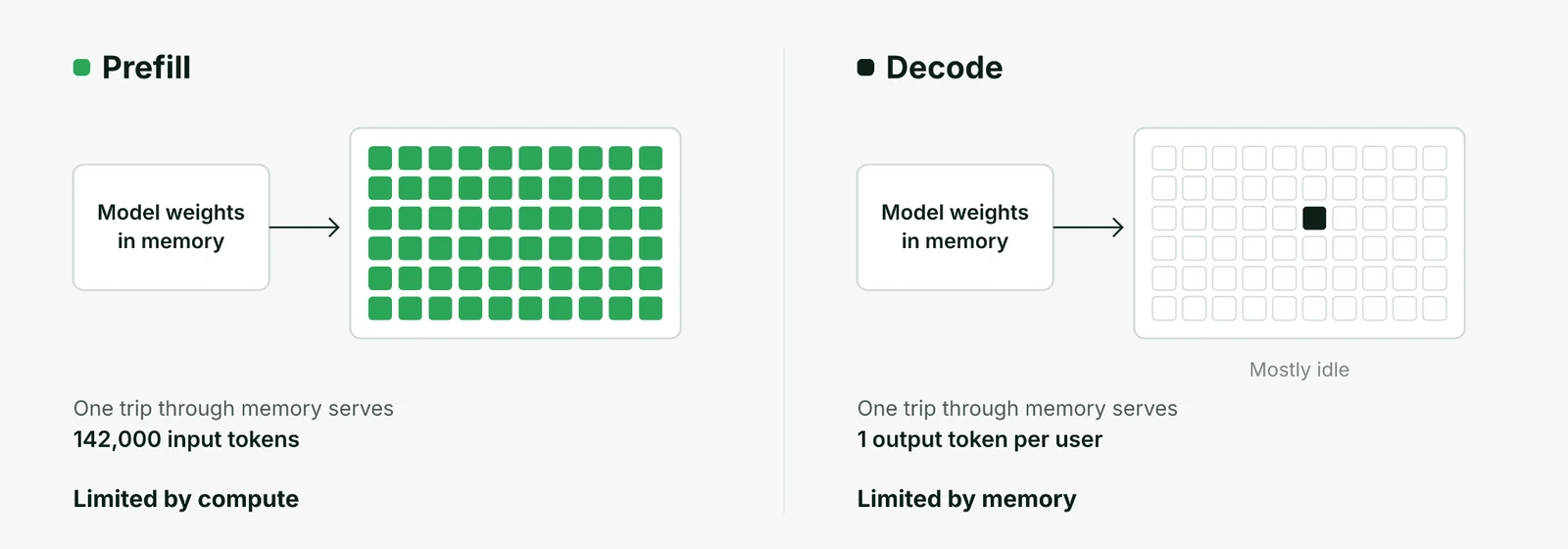
Figure 2: In prefill, one trip through memory serves every input token. In decode, the same trip serves one output token per user, so the arithmetic units mostly wait.
Decode can’t work that way. Each output token depends on the one before it, so the model must compute them one at a time. Therefore, every output token needs its own full pass through the weights: a 1,100-token answer means streaming the weights 1,100 times, each pass producing just one token per user.
For this reason, during decode, the arithmetic units spend much of each pass waiting for weights to arrive. In the very low batch size regime, such as serving a single user, an NVIDIA B200 can leave its arithmetic units idle more than 99% of the time.
Serving many users at once helps, because each trip through memory then produces one token for every user in the batch. Techniques such as speculative decoding, which checks several draft tokens in one pass, also help. But neither removes the bottleneck. Each user also needs room in GPU memory for conversation data, which caps how many users can share each pass.
Memory, both its bandwidth and its capacity, sets the pace of decode.
Disaggregated Inference: The Central Planning Question
As shown, the speed of each inference job depends on different hardware resources. For that reason, many large operators now run them on separate GPU pools, each optimized differently. DeepSeek, for example, runs prefill on units of 4 servers and decode on units of 18 servers. This technique is called “disaggregated inference.”
At scale, a cluster serves hundreds of requests at once, each at a different stage. At any moment, the prefill pool reads new user prompts while the decode pool writes answers for requests that finished prefill earlier. Since every request passes through both pools, the cluster can run only as fast as the slower one.
That constraint raises the main planning question of fleet design at scale. Assuming a fixed budget, how many GPUs should each pool get?
What Real AI Traffic Looks Like
The natural place to look for an answer is the traffic itself, and today's AI traffic reads far more than it writes.
For example, SemiAnalysis created its AgentX benchmark by replaying 393 real Claude Code sessions. In that dataset, the median request carries 142,016 input tokens and 444 output tokens. This article's example uses 142,000 input tokens and a longer 1,100-token answer. The longer answer adds decode work, so it understates prefill's share rather than inflating it.

Figure 3: Token mix for one agentic coding turn in this article's example, with about 142,000 input tokens and about 1,100 output tokens.
At first glance, the sizing answer looks obvious. If roughly 99% of tokens are input, an operator should put nearly the whole fleet on prefill.
However, that conclusion turns out to be wrong.
Most of Each Prompt Is Old News
The reason lies in how people actually use AI tools: most serious work happens in multi-turn sessions, not single questions.
Consider a developer working with a coding agent. On the first turn, the agent reads the codebase. On the second turn, the application sends the entire conversation again, plus the developer's new request. By turn five, the prompt holds turns one through four plus a few new lines.
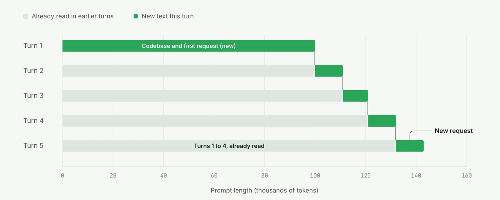
Figure 4: In a multi-turn session, each prompt repeats everything from earlier turns. Token counts are illustrative.
In other words, most of each new prompt is text the model has already read. Reading it again from scratch would repeat the same prefill work every turn. Operators exploit this feature by saving and reusing the model's work from earlier turns.
That saved work is called the “KV cache.” During prefill, the model records what it computes for each input token. When the next turn starts with the same text, the serving system loads those records instead of computing them again from zero. That way, only the new part of the prompt needs prefill.
For example, a developer might ask an agent to refactor a module, step away for 30 minutes, then return with a follow-up. If the serving system still holds that session's KV cache, the agent picks up where it left off. If not, the agent has to read the entire codebase again at full cost.
Cache Hit Rate: A Number That Changes the Math
The “cache hit rate” is the share of input tokens the system successfully loads from the cache, instead of computing from scratch. For a hit to occur, the system must still have that text’s KV cache stored when the user returns, rather than evicting it in the interim.
In practice, real workloads reuse most of their input. Requesty, an LLM routing service, reported a 92% prompt-cache hit rate for Claude Code traffic in April 2026. In SemiAnalysis's AgentX runs on NVIDIA B300 systems, 91% of prompt tokens came from cache held in GPU memory. And Character.AI has reported a 95% cache rate for chat with long histories. Even across all of DeepSeek’s V3 and R1 traffic over one day in February 2025, 56% of input tokens hit its on-disk KV cache.
Those hit rates change how we see the 99% figure. At a 95% cache hit rate, a 142,000-token prompt needs only about 7,100 tokens of fresh prefill. The serving system loads the other 134,900 tokens from the cache. Caching therefore shrinks the input-to-output token ratio from about 130:1 to about 6:1.
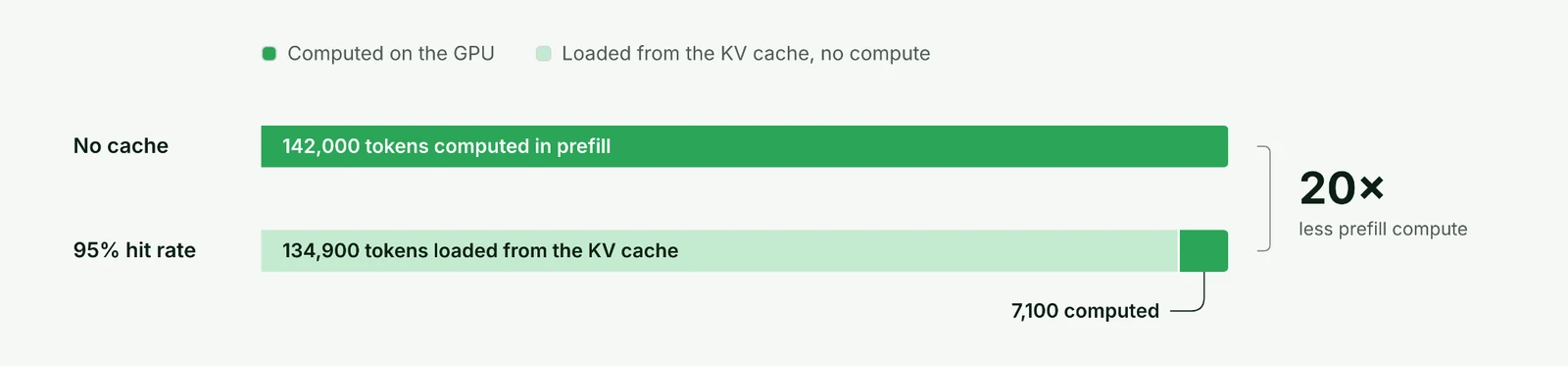
Figure 5: The same 142,000-token prompt with no cache and with a 95% cache hit rate.
Caching doesn’t make that work free, though. Instead of recomputing the prompt, the system has to keep the earlier results.
This article's example assumes a large mixture-of-experts model similar to GLM-5.2, storing about 48 KB of KV cache per token. At that size, one 142,000-token session produces about 6.8 GB of KV cache. Between turns, the system must store that 6.8 GB somewhere and reload it when the user returns. So each cache hit saves GPU computation, but the system pays for it in storage space and in the time spent moving data back.
How Hit Rate Reshapes a 1,000-GPU Fleet
To see how much that trade matters, consider a cluster of 1,000 B200 GPUs serving agentic coding traffic. Assume each turn carries 142,000 input tokens and produces about 1,100 output tokens.
According to ElastixAI's modeling, one B200 prefills about 25,000 input tokens per second. When decoding long agentic sessions, one B200 produces about 1,000 output tokens per second across all users.
With no caching, each turn costs about 5.7 GPU-seconds of prefill and 1.1 GPU-seconds of decode. Prefill takes 84% of the work, so the right design puts about 840 GPUs on prefill and 160 on decode. Sized that way, the cluster serves about 147 turns per second.
At a 96% cache hit rate, prefill drops to about 0.23 GPU-seconds per turn, while decode remains constant. Prefill now takes only 17% of the work, so the right split flips to about 170 prefill GPUs and 830 decode GPUs. The same 1,000 GPUs then serve about 750 turns per second, five times more.
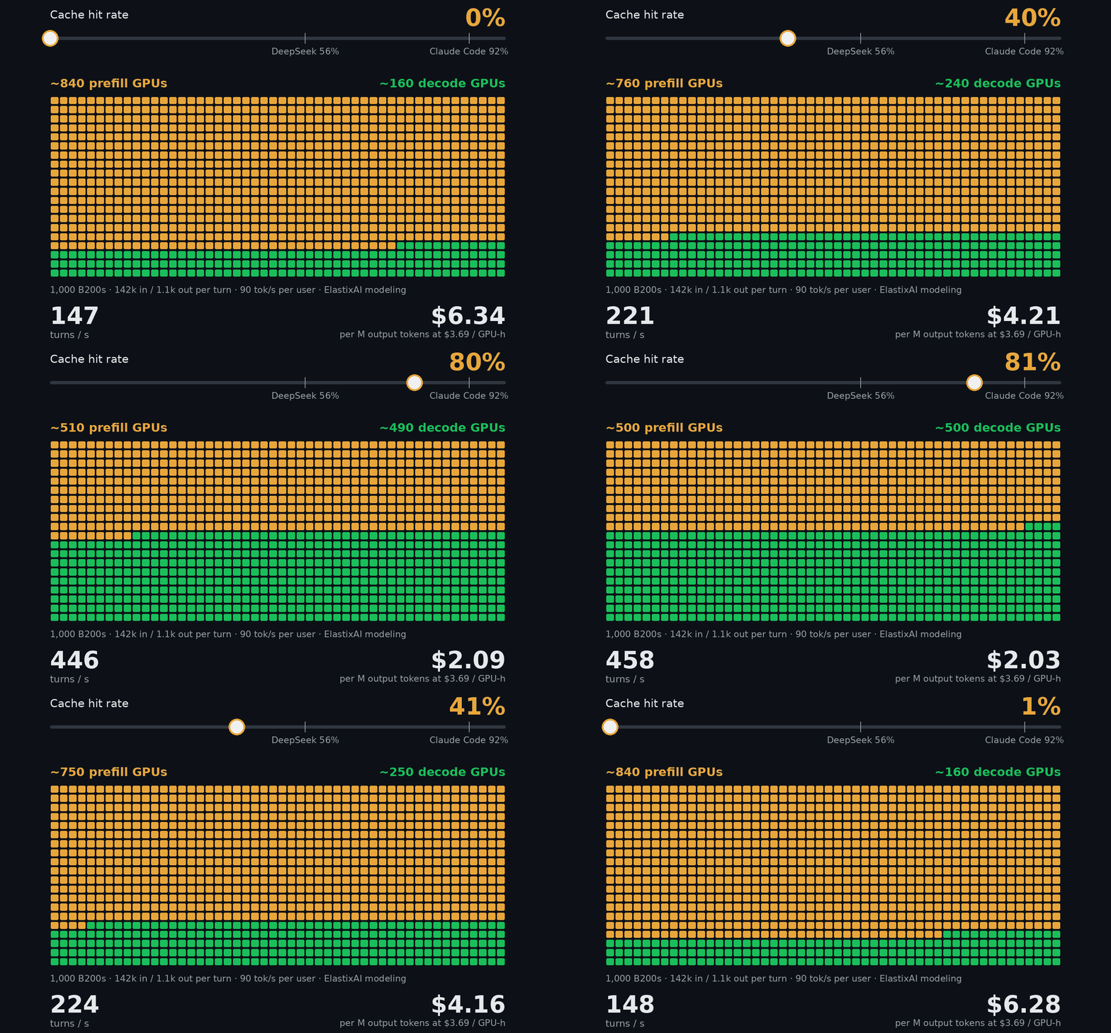
Figure 6: Traffic shape sizes the fleet and, in turn, drives cost per output token. Model: 1,000 B200s, 142,000 input and 1,100 output tokens per turn, 25,000 prefill tokens per second per GPU, and 1,000 decode tokens per second per GPU (about 11 sessions at 90 tokens per second each), $3.69 per GPU-hour.
The economics are equally impacted. At $3.69 per GPU-hour, cost per million output tokens falls from about $6.34 to about $1.24. That price is the lowest on-demand B200 rate among the 31 cloud providers American Compute tracks. At the $6.82 median price, both figures nearly double, but the five-fold difference remains.
Planning for Hit Rate
Given the huge impact of cache hits, operators should plan their GPU allocation around it. The catch is that operators can’t always rebalance a fleet quickly. Once they assign GPUs to each pool, the fleet performs well only near the planned hit rate.
Take a fleet sized for no caching, with 840 prefill GPUs and 160 decode GPUs. If the hit rate climbs to 96%, prefill work shrinks. But without a way to use this gain, the 160 decode GPUs still finish only about 147 turns per second, and most of the prefill pool sits idle.
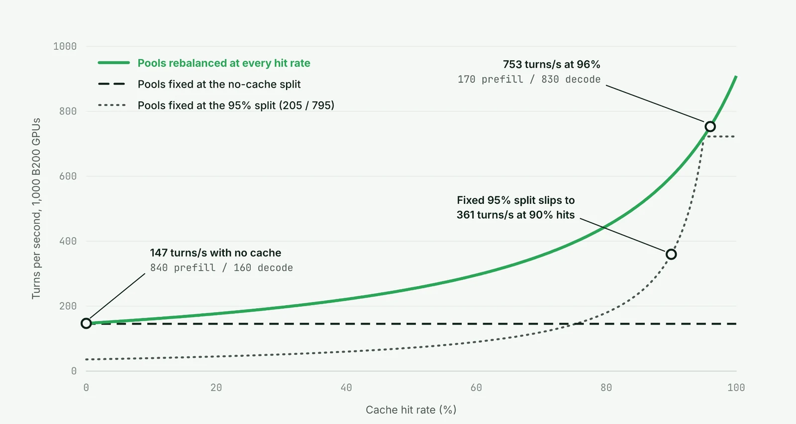
Figure 7: Throughput of 1,000 B200 GPUs on agentic coding traffic at each cache hit rate. A fixed split performs well only near the hit rate it was sized for. Source: ElastixAI modeling.
The reverse case is more surprising. A fleet sized for 95% hits has about 205 prefill GPUs and 795 decode GPUs, and it serves about 722 turns per second.
If the hit rate slips to 90%, the uncached share of each prompt goes from 5% to 10%. A five-point drop in hit rate sounds small, but it doubles the tokens the prefill pool must process, from about 7,100 to about 14,200 per turn. The same 205 prefill GPUs can now handle only about 361 turns per second, down from about 722. The decode pool could still handle 722, but it only receives what prefill finishes, so half of it waits idle.
In other words, hit rate decides the right layout more than the model does. That finding raises the next question: what decides the hit rate?
Storage Sets the Hit Rate
A returning user gets a cache hit only if the serving system still holds that user's KV cache. Whether it does depends on storage.
GPU memory is too small and too expensive to hold every idle session. So between turns, the serving system moves caches out to larger, slower tiers. These tiers include the server's DRAM, local flash drives, and shared network storage. Meanwhile, new sessions keep arriving and push older ones out.
Each tier therefore holds a session for roughly its capacity divided by the rate of new cache data.
In the 96% example, each eight-GPU server writes about 2 GB of new cache data every second. At that rate, the 2 TB of DRAM in an NVIDIA DGX B200 holds a session for about 17 minutes. That window covers the short pauses inside an agent loop. The 30 TB of flash in the same server holds a session for a window of about four hours. Keeping sessions overnight would take 120 to 250 TB per server.
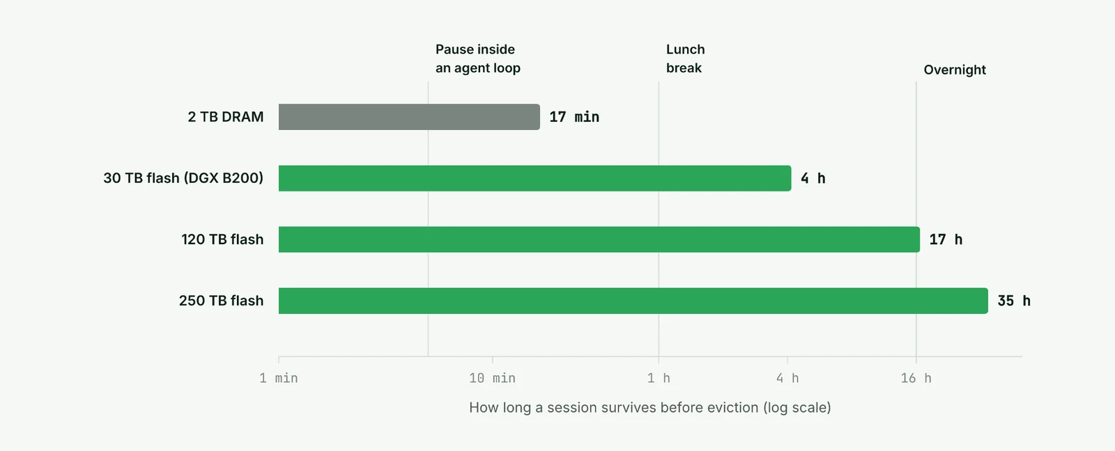
Figure 8: How long each storage tier holds a session at a 96% hit rate, with about 2 GB/s of new cache data per eight-GPU server. Idle gaps are typical values, not measurements.
When a user returns after the window closes, the system misses and reads the whole prompt again at full cost. Misses also feed on themselves. Each miss creates a fresh cache that takes up storage, pushes other sessions out sooner, and causes more misses.
Put together, these effects form a single chain. Storage capacity sets how long sessions survive. Session survival sets the hit rate. The hit rate determines how many output tokens each GPU can produce, and AI providers ultimately sell output tokens.

Figure 9: At scale, storage capacity sets an upper bound on hit rate, output tokens, and revenue.
That chain leads to this article's central finding.
Within a fixed fleet, GPUs can produce only as much as the slower pool allows. Take the fleet sized for 95% hits from earlier. If its storage can’t hold sessions long enough and the hit rate slips to 90%, its 205 prefill GPUs cap throughput at about 361 turns per second. Adding decode GPUs changes nothing, because they only receive what prefill finishes.
Even with the pools rebalanced, raising the hit rate does more than adding GPUs.
At a 90% hit rate, the 1,000-GPU cluster serves about 600 turns per second. Raising the hit rate to 96% lifts that to about 750, with no new GPUs. Reaching 750 turns per second at 90% would instead take about 1,260 GPUs, roughly 260 more.
Importantly, operators raise the hit rate with capacity. Each tier holds sessions for its capacity divided by the rate of new cache data, so doubling a tier’s capacity doubles how long it keeps each session.
The point? For a cluster serving long, multi-turn sessions, adding memory and storage can raise throughput far more effectively than adding GPUs.
Put more simply: at scale, AI inference is as much a memory and storage problem as a compute problem.
Planning Infrastructure Around How People Use AI
AI usage is shifting toward longer, multi-turn agent sessions, and that shift makes the opening question harder to answer. Teams can no longer size a fleet from the model alone. The right layout depends on how often users return, how long they stay away, and how much storage holds their sessions in between.
For infrastructure teams, that reality changes how planning works. Hit rate deserves the same attention as model choice, and teams should measure it on their own traffic before they buy hardware. Storage belongs in the first conversation about a fleet, not the last.
A new agent framework or a longer context window can also move the hit rate within months. Teams should expect the right split between prefill and decode to move with it.
That pace of change favors hardware that can adapt. Fixed-function silicon locks in one compute-to-memory ratio for years, while the workload can reshape within weeks. When hardware is software-defined and reconfigurable, operators can retune it as models, context lengths, and hit rates shift, instead of waiting for the next purchase cycle.
In an industry where memory and storage increasingly decide output, hardware that adapts to the workload will make more of every dollar and every watt.